Wednesday 19 December 2007

Matplotlib tips

Recently I've been doing some plots with matplotlib. Although it has all gone well, it hasn't been entirely obvious how to do certain things. So, for the benefit of posterity (i.e. me in a month's time) I'm going to record some of my newly-gained knowledge here.
  • Colours: 'gray' is a colour too, 'k' is short for black.
  • Don't like the border on a legend? You need to stick the legend into a variable, "leg = legend()" for example, and say "leg.draw_frame(False)" (this pearl of wisdom comes courtesy of the matplotlib source code).
  • Want to make the legend text (and hence the legend) smaller? Try legend(prop={"size":10}).
  • To adjust the position or font of text in a plot, it may be easiest to save as SVG, open in Inkscape (a truly fantastic program), click on the image and hit 'Ungroup' a few times (CTRL+SHIFT+G), make the adjustments, resave the SVG, and finally Export to Bitmap (300 dpi is probably good enough).
  • Want two overlapping histograms on the same plot? Use the width keyword to hist() to set the bar widths to half the bin size. Also, catch the rectangles used to make the second histogram so that you can offset the bars by adding half the bin size:

    a, b, c = hist(x, bins, facecolor='k', width=width)

    for rect in c:
    rect.set_x(rect.get_x() + width)
    Update 11/05/2010: With current version of Matplotlib, you need to replace width=width with rwidth=0.5.
    You might also want to store the first rectangle of each histogram in a list and pass it as a first argument to legend.
  • To add a regression line between x=100 and x=600 (and get the R and significance values for free), try:

    from scipy import stats
    grad, inter, r, p, std_err = stats.linregress(x, y)
    plot((100, 600), [grad*x + inter for x in [100, 600]])
  • Line styles: "-" for solid, "--" for dashed, ":" for dotted. Unfortunately, the gaps in 'dashed' are too big. To define your own line style, you need to catch the line in a variable, e.g. "lines = plot(...)", and use lines[0].set_dashes((5,2)) for dashes of length 5 separated by gaps of 2 (unknown units).
  • Want Greek symbols and subscripts in axes labels? It worked for me on windows with something like the following:

    rc('text', usetex=True)
    xlabel(r"$\rho_{8.0}", fontsize="large")
    Note that the first time you run this on Windows, matplotlib might need to connect to the internet to download a needed component (MiKTeX). Also, when you make changes to the TeX stuff you might need to run your program twice to pick up on the changes.
    Update 03/01/2011: With current version of Matplotlib, a TeX parser is included.
    The Angstrom symbol can be include in a legend as follows: "RMSD ($\AA$)". For more information on available symbols, see the Matplotlib mathtext page.

Wednesday 12 December 2007

Using Jmol for Drug Design - Depict Ligand in Active Site

In the previous article, I showed how to install Jmol. This article will look at depicting a ligand in a protein active site with a few extra complications. This example was not chosen to showcase Jmol - this is a real-life example of a figure I need to create. You can find on the web lots of examples of scripting Jmol to turn on/off ball-and-stick models. Figuring out how to do difficult things is a bit harder, and I hope others will find this example useful...

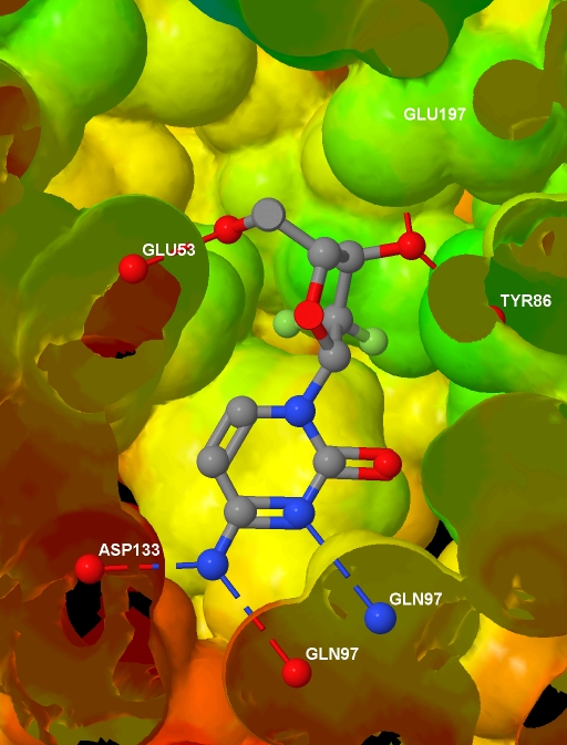
Specifically, I want to depict the ligand in the protein active site, with the protein represented by an isosurface coloured by depth in the protein (values which I will supply), and with protein-ligand hydrogen bonds shown. I have a protein .MOL2 file with hydrogens added; I have a ligand .MOL file, I have the corresponding protein .PDB file (no hydrogens and the ligand and waters have been removed); and I have a text file containing, for each atom in the protein .MOL2 file, a value related to the depth of that atom in the protein. And here is the final image (screenshotted from the browser , cropped a little, and saved as a JPG with zero compression - click for the original image):Before presenting the necessary code, to help understanding I note that Jmol imposes some constraints:
  • bonds can only exist between molecules in the same model
  • if the slab is turned on, it cuts through every model
  • Jmol can identify the residue names in the PDB file, but not in the .MOL2 file
  • Jmol does not automatically identify protein-ligand hydrogen bonds
  • if mapping property data onto an isosurface, it needs to be supplied for every atom in the model (actually, there is an alternative, but this is a good rule of thumb)
I should also point out that Jmol can colour isosurfaces by depth in the protein automatically, but I wanted to use my own measure of depth. Update 13/12/07: Due to popular demand, here is the actual applet in motion: [low quality] [high quality]. And finally, after all that, here is the code (available also as a download):
<html>
<head>
  <script type="text/javascript" 
  src="file:///D:/Tools/Jmol/jmol-11.3.53/Jmol.js">
  </script>
  </head>
<body>
<script type="text/javascript">
  var protein = "1p62";
  jmolInitialize("file:///D:/Tools/Jmol/jmol-11.3.53", true);
  var jmolcmds = [
  // Load the molecules
  "load file:///D:/Ligands/" + protein + "_ligand.mol",
  "set appendNew = false",
  "load APPEND file:///D:/Proteins/" + protein + "_protein.mol2",
  "set appendNew = true",
  "load APPEND file:///D:/Proteins/" + protein + ".pdb",

  // Turn up display quality but don't yet show anything
  "display none; set antialiasDisplay true",

  // The following is the output of "show orientation"
  "reset;center {67.99645 35.5767 19.92025}",
  "rotate z -21.47; rotate y 25.81; rotate z 74.65",
  "zoom 400.0; set rotationRadius 35.03",

  // Add the HBonds
  "model 1.1",
  "connect 3.1 (molecule=1 and elemno=8) \
(molecule!=1 and elemno=7) HBOND RADIUS 0.07 CREATE",
  "connect 3.2 (molecule=1 and elemno=7) \
          (molecule!=1 and elemno=8) HBOND RADIUS 0.07 CREATE",
  "connect 3.1 (molecule=1 and elemno=8) \
(molecule!=1 and elemno=8) HBOND RADIUS 0.07 CREATE",
  "connect 3.1 (molecule=1 and elemno=7) \
(molecule!=1 and elemno=7) HBOND RADIUS 0.07 CREATE",

  // Load info for isosurface and draw it
  "{model=1.1}.property_d = load(\"D:/Data/" + protein +"_rd.txt\")",
  "isosurface select(molecule!=1 and within(10.0, molecule=1)) \
ignore(molecule=1) resolution 5 sasurface 0 \
COLOR ABSOLUTE 30 120 REVERSECOLOR MAP property_d",

  // Select and label the HBonded protein atoms in model 2.1
  "define hbondedproteinatoms within(3.2, true, \
model=1.1 and molecule=1 and (elemno=7 or elemno=8)) \
and not within(0.1, true, model=1.1 and molecule=1) \
and model=2.1 and not elemno=1 and not solvent",
  "select hbondedproteinatoms; font label 15 SANSERIF BOLD",
  "set labelFront; color label white; label %n%R",

  // Add to selection the ligand and
  // its HBonded protein atoms in model 1.1
  "select selected or (((molecule=1 and model=1.1) or \
within(3.2, molecule=1 and model=1.1 and \
(elemno=7 or elemno=8))) and not elemno=1)",

  // Slice through everything with a slab
  "slab on; slab 51",

  // Remove the Jmol logo (I will reference Jmol instead)
  "set frank off",

  // Show the selected data from all models
  "model 0; display selected",
  ];
  jmolApplet(700, jmolcmds.join("; "));
</script>
</body>
</html>

Tuesday 11 December 2007

Using Jmol for Drug Design - Installation

Jmol is well known as the program for showing 3D structures in webpages. It's free, it's open source and it has excellent support. However, I've often felt that Jmol's potential is not being fully realised by chemists in general, and by me in particular. So this series of posts will describe how to use Jmol to create publication quality pictures of drug molecules in a protein active site. More about that in the next post; first we have to install Jmol.

I'm going to be running Jmol as an applet in Firefox on my Win XP machine. Note that Jmol also comes as a stand-alone application. The benefit in running Jmol in a web browser is that you have access to the JavaScript scripting language. The only downside is that you need to remember to use the signed applet (as described below) or else you will have problems opening files at arbitary locations on your computer.

Step one is to download the absolutely latest Jmol. If you look at the download page, see under Jmol Prerelease Tests for the cutting edge (currently 11.3.54). There's a new version practically every day. The file you want is called something like jmol-11.3.54-binary.zip. Download and unzip the file into something like D:\Tools\Jmol\jmol-11.3.54.

Next, download the protein structure 1hnn from the PDB and save as something like D:\Proteins\1hnn.pdb.

Now we can create the "Hello World" of Jmol applets, which simply loads and displays the protein structure you have just downloaded. Save the following code as something like D:\Applet\HelloWorld.htm. You should change the paths in the following HTML to correspond to the actual paths on your computer:
<html>
<head>
<script type="text/javascript"
src="file:///D:/Tools/Jmol/jmol-11.3.54/Jmol.js">
</script>
</head>
<body>
<script type="text/javascript">
jmolInitialize("file:///D:/Tools/Jmol/jmol-11.3.54", true);
var jmolcmds = [
"load file:///D:/Proteins/1hnn.pdb",
];
jmolApplet(700, jmolcmds.join("; "));
</script>
</body>
</html>

Open the HTML file with Firefox. The first time you do this, you will be asked whether you trust Jmol to access your hard drive responsibly. You should say yes to this if you wish to proceed. This warning indicates that you are using the signed applet rather than the unsigned applet. Using the signed applet on a live website will probably discourage users, so is best avoided, but it is very useful when running locally on your machine, as the unsigned applet is restricted to opening files in particular directories.

The next post takes Jmol to the next level, uh, level 2.

Wednesday 5 December 2007

Python gives you wings

Along with Piled Higher and Deeper, I really like xkcd. Today's comic is on a theme close to my heart:To pander to the readership of this blog, here's one on a more popular scripting language: