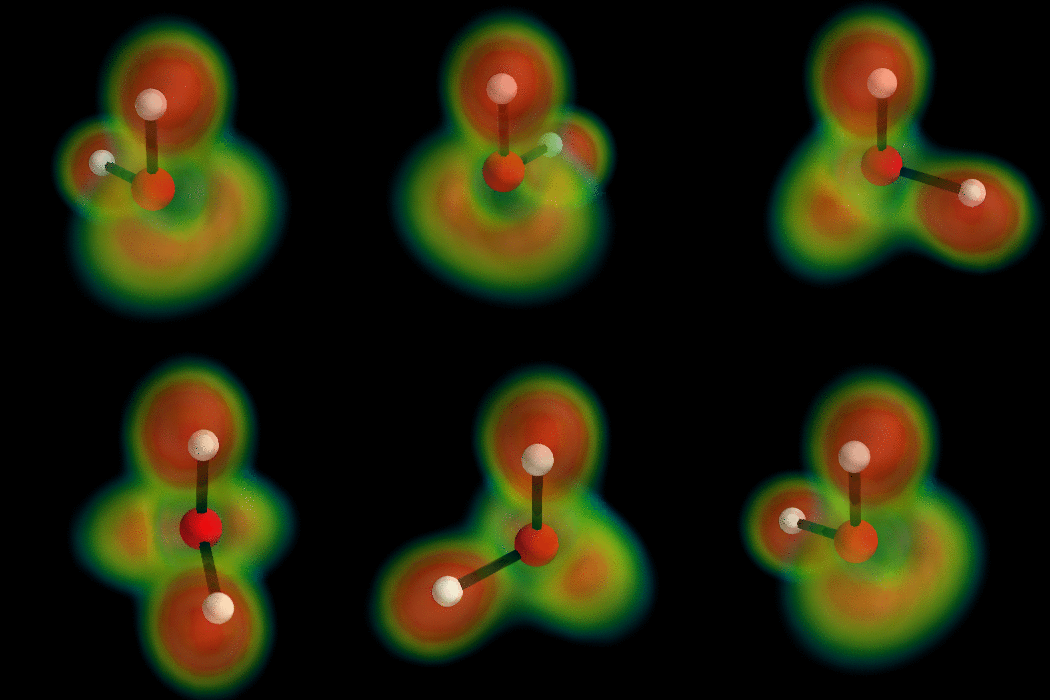
There's no need for us to keep drawing isosurfaces for the electron density and other volumetric data generated by QM calculations. Driven by the engineering field, there are a couple of really amazing open source visualisation toolkits out there that we can use to do so much more. One of these is the
VTK.
David Lonie, as part of Google Summer of Code with
Marcus Hanwell of VTK/Avogadro as mentor, is integrating aspects of the VTK into Avogadro (see
this post for example). But I can't wait, so I've busted out the VTK myself and now present the ELF of water:

To generate this type of image, install
Mayavi2 (not exactly trivial to be honest), and then run the following Python script to generate PNG files (this script is adapted from
a Mayavi example, which you may want to run first):
"""
In this example, we display the H2O molecule, and use volume rendering to
display the electron localization function.

The atoms and the bounds are displayed using mlab.points3d and
mlab.plot3d, with scalar information to control the color.

The electron localization function is displayed using volume rendering.
Good use of the `vmin` and `vmax` argument to
`mlab.pipeline.volume` is critical to achieve a good visualization: the
`vmin` threshold should placed high-enough for features to stand out.

The original is an electron localization function from Axel Kohlmeyer.
"""
# Author: Gael Varoquaux <gael.varoquaux@normalesup.org>
# Copyright (c) 2008, Enthought, Inc.
# License: BSD Style.
# Edited by: Noel O'Boyle <baoileach@gmail.com>

# Retrieve the electron localization data for H2O ##############################
import os
if not os.path.exists('h2o-elf.cube'):
    # Download the data
    import urllib
    print 'Downloading data, please wait'
    opener = urllib.urlopen(
        'http://code.enthought.com/projects/mayavi/data/h2o-elf.cube'
        )
    open('h2o-elf.cube', 'wb').write(opener.read())


# Plot the atoms and the bonds #################################################
import numpy as np
from mayavi import mlab
mlab.options.offscreen = True
mlab.figure(1, bgcolor=(0, 0, 0), size=(350, 350))
mlab.clf()

# The position of the atoms
atoms_x = np.array([2.9, 2.9, 3.8])*40/5.5
atoms_y = np.array([3.0, 3.0, 3.0])*40/5.5
atoms_z = np.array([3.8, 2.9, 2.7])*40/5.5

O = mlab.points3d(atoms_x[1:-1], atoms_y[1:-1], atoms_z[1:-1],
                  scale_factor=3,
                  resolution=20,
                  color=(1, 0, 0),
                  scale_mode='none')

H1 = mlab.points3d(atoms_x[:1], atoms_y[:1], atoms_z[:1],
                   scale_factor=2,
                   resolution=20,
                   color=(1, 1, 1),
                   scale_mode='none')

H2 = mlab.points3d(atoms_x[-1:], atoms_y[-1:], atoms_z[-1:],
                   scale_factor=2,
                   resolution=20,
                   color=(1, 1, 1),
                   scale_mode='none')

# The bounds between the atoms, we use the scalar information to give
# color
mlab.plot3d(atoms_x, atoms_y, atoms_z, [1, 2, 1],
            tube_radius=0.4, colormap='Reds')

# Display the electron localization function ###################################

## Load the data, we need to remove the first 8 lines and the '\n'
str = ' '.join(file('h2o-elf.cube').readlines()[9:])
data = np.fromstring(str, sep=' ')
data.shape = (40, 40, 40)

source = mlab.pipeline.scalar_field(data)
min = data.min()
max = data.max()
vol = mlab.pipeline.volume(source, vmin=min+0.65*(max-min),
                                   vmax=min+0.9*(max-min))

mlab.view(132, 54, 45, [21, 20, 21.5])

##mlab.show()

f = mlab.gcf()
for i in range(36):
    f.scene.camera.azimuth(10)
    f.scene.render()
    mlab.savefig('example_%02d.png' % i)
To create an AVI from these PNGs, use mencoder:
C:\Tools\mayavi>..\MPlayer-p4-svn-33883\mencoder.exe "mf://example_%02d.png" -mf fps=10 -o anim.avi -ovc lavc -lavcopts vcodec=msmpeg4v2:vbitrate=500
To create an animated GIF use ImageMagick:
C:\Tools\mayavi>convert -delay 10 -loop 0 example_*.png animation.gif
